Continuing with my exploration of MATLAB/Arduino interfacing, this post examines two methods of removing noise from sensor data: exponential moving average and simple moving average filters. As a precursor to this, an introduction to serial communication and data plotting with Arduino and MATLAB can be found on my previous post. All the code used in these posts is available at my GitHub repo. Again, I am using the tutorial videos from matlabarduino.org as a reference, while adding my own features/improvements along the way.
Exponential moving Average (EMA)
The exponential moving average is assigns a weighting factor, with the most recent data having the largest weight. It is computed by the following equation:
$$gX_{filt} = (1-\alpha)*gX_{filt-old}+\alpha*gX_{raw}$$ $$\alpha\in\left[0,1\right]$$
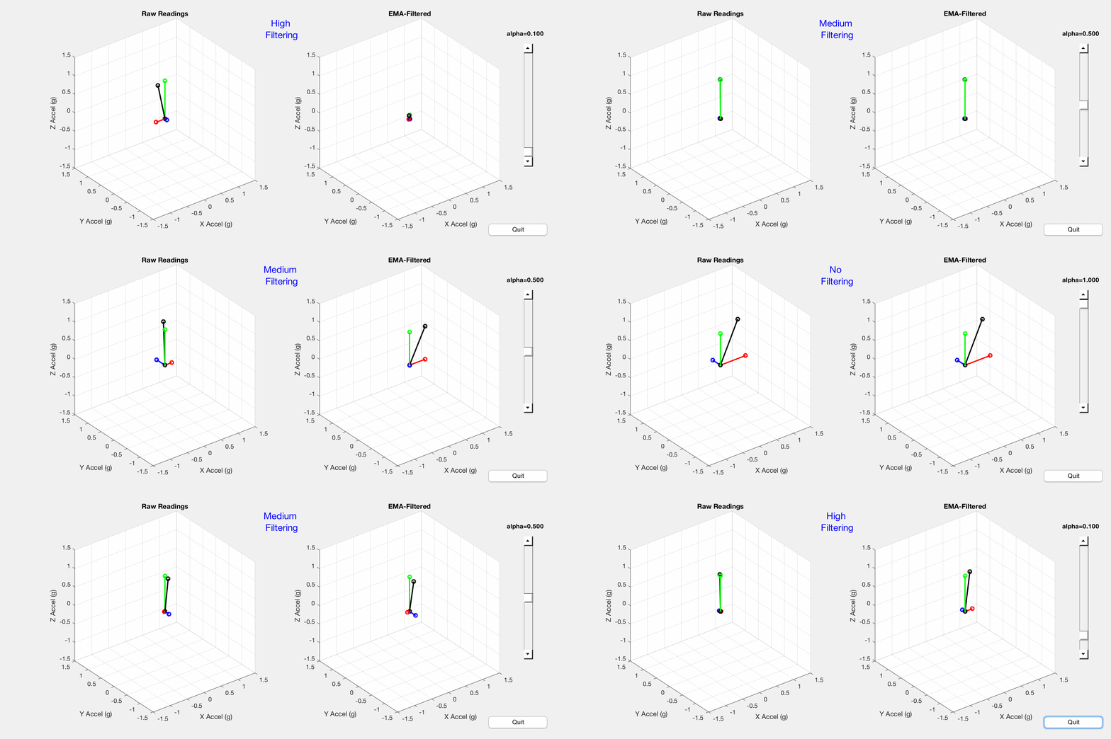
Per my previous post, the LSM303DLHC accelerometer is interfaced with an Arduino Uno, serial communication between Arduino and MATLAB is established, and MATLAB plots the gravitational acceleration vectors. Previous MATLAB code is modified to calculate the EMA and display side-by-side plots of raw and filtered data. The result is pictured below — notice the difference between raw and filtered data as the slider changes the alpha value.
Comparison of raw (left) and EMA-filtered (right) acceleration vectors.
In the graphic above, the accelerometer is held in space with the z-vector perpendicular to earth. Movement and vibration are applied to the accelerometer to show response to sudden changes in orientation. In comparing the raw data on the left with the filtered data on the right, the following observations are made:
- Alpha value approaching 1 results in high-filtering — the filtered plot moves very little in response to movement.
- Alpha value approaching 0 results in low-filtering — there is little difference between raw and filtered plots.
- Alpha value around 0.5 provides an optimal level of filtering — the filtered plot is free of erratic jitter and responds to movement.
simple moving average (sma)
As the name implies, this filter employs a simple average to incoming sensor data. With each iteration of the code-loop, the oldest value in the data-set is dropped out and replaced with the latest reading, and a new average is computed. The SMA is given by the following equation where the level of noise-reduction is determined by n (the number of 'taps').
$$gX_{filt} = \frac{gX_{i}+gX_{i-1}+\ldots+gX_{i-(n-1)}}{n}$$
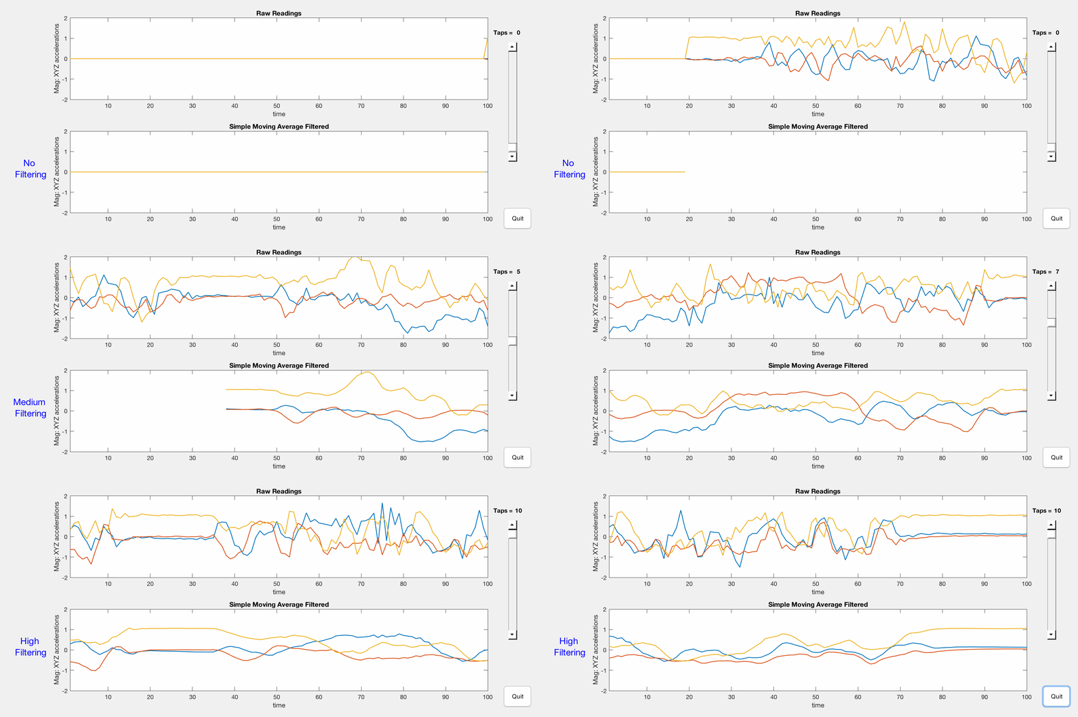
The magnitudes of x/y/z-axis accelerations are visualized in 2D plots using MATLAB. Both raw and filtered data are presented, and a slider is used to adjust the amount of filtering (number of taps).
Comparison of raw (top) and SMA-filtered (bottom) x/y/z acceleration magnitudes.
The accelerometer is manipulated in the same manner as with the EMA filter. To summarize the effects of the SMA filter:
- Zero taps = no filtering — raw accelerometer readings reveal high sensitivity to slight perturbations.
- Ten taps = high filtering — vigorous accelerometer movement is unseen in filtered results.
- Five taps = optimal filtering — jitter is eliminated, yet filtered results reflect large movements.
conclusion
I am now fairly competent with using MATLAB for sensor characterization and will be utilizing this in future projects. What immediately comes to mind is applying this in the observation/definition of thresholds when using accelerometers in robotics/automotive applications. One example is the improvement made on impact-detection by filtering erroneous jitter introduced by body vibrations.

